Migrated and Ready to Ship? I Hit PostgreSQL with 150 Connections, Created 180,000 Dead Tuples, Then Recovered an Accidental DELETE

TL;DR

Migrating from MySQL to PostgreSQL, reconciling the data, and tuning the parameters still do not prove that the new database is ready to launch. Production readiness requires you to hit at least four walls yourself: what happens when connections are exhausted, whether slow SQL can be found through an evidence chain, whether dead tuples are reclaimed in time, and whether an accidental deletion can be recovered to the correct moment. I ran a destructive rehearsal in a PostgreSQL 18.6 sandbox that publishes no host ports and contains only synthetic data. One hundred and fifty direct clients produced too many clients; the same 150 clients behind PgBouncer used about 21 database backends, completed 35,751 transactions, and failed zero; one query fell from 61.953ms to 2.153ms; 180,000 dead tuples became zero after an ordinary VACUUM; and a deleted row came back through a base backup plus 22 archived WAL files. This is the finale of my PostgreSQL series, with one-click labs for Windows 11, Ubuntu 26.04, and macOS 26, plus a bounded prompt for Agent-driven execution.

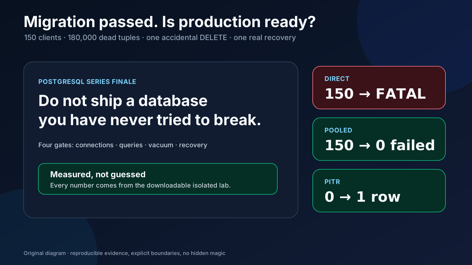
Figure 1: Original SVG cover. Every number comes from the downloadable isolated lab. None is a capacity promise or a benchmark borrowed from someone else’s machine.

1. Why Does This Series Need a Finale?

The first three parts answered three different questions. Part one explored why projects move from MySQL to PostgreSQL. Part two performed and verified a MySQL-to-PostgreSQL migration. Part three turned ten production switches that matter after the move.

All three were missing the final verb: prove.

Think of moving a hospital from an old building into a new one. Every medical record has arrived, the lights work, and the air conditioning is tuned. That still does not mean the hospital should admit patients tomorrow. Someone must cut the power and watch the generator take over. Many people must try to register at once so the team can see whether the front desk collapses. Someone must deliberately retrieve the wrong record and prove that the right version can be restored. A database launch is the same: a configuration sheet says, “we think this should work”; a failure rehearsal says, “the evidence shows what it actually does.”

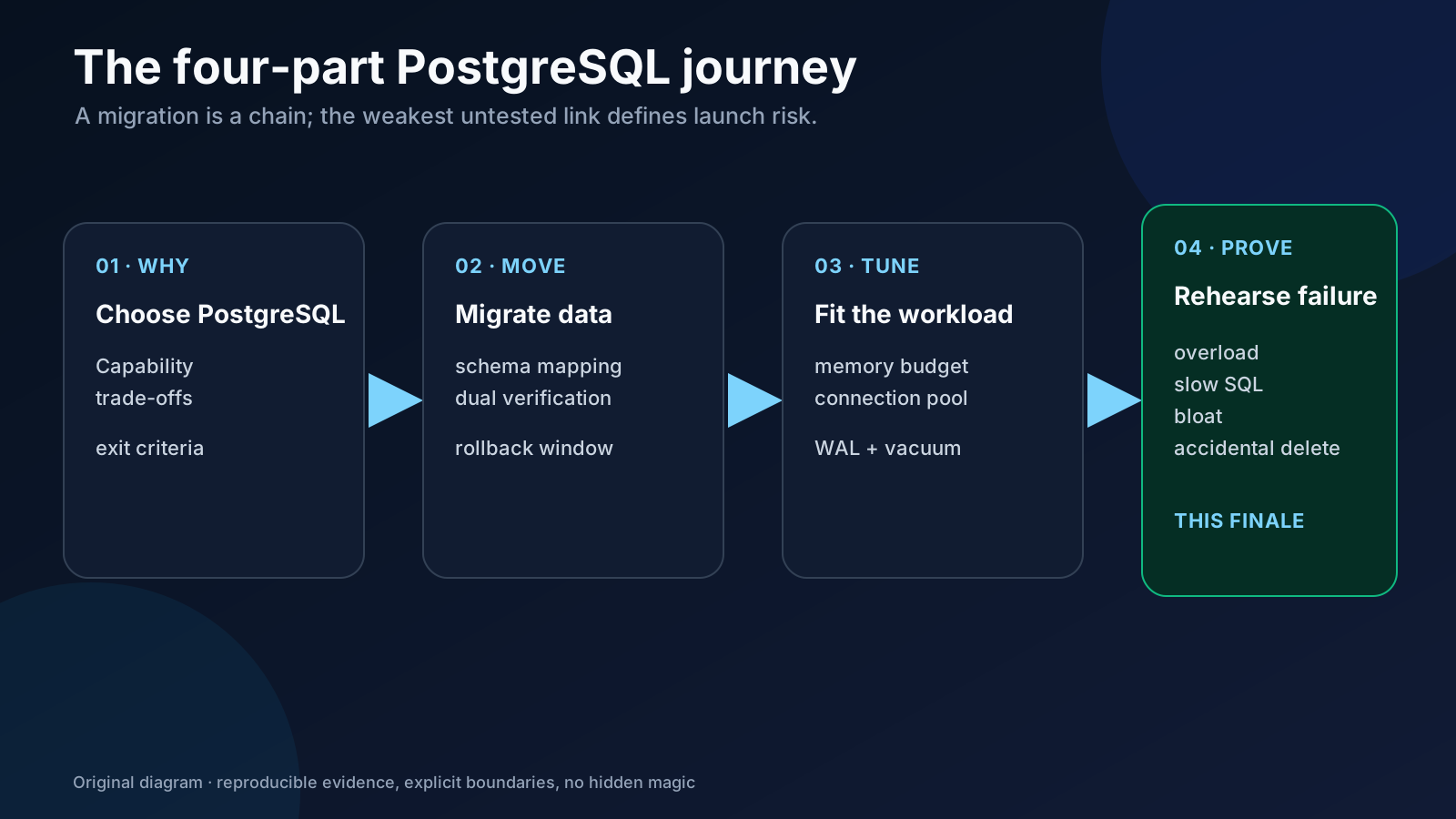
Figure 2: Original diagram. Selection, migration, tuning, and proof are not four unrelated posts. They form one chain, and an untested final link can erase the success of the first three on launch day.

This article does not pretend that a small sandbox is a production capacity test. The lab answers narrower, useful questions: does the pool really fold clients into fewer backends, does the execution plan really change, does VACUUM really make dead space reusable, and does PITR really retrieve data committed before a target time? A real launch still needs another rehearsal with the real data distribution, connection lifecycle, query mix, and storage system.

2. Symptoms: Four Problems That Hide Until Launch Day

2.1 The 101st Guest Blocks the Door

PostgreSQL uses one backend process per connection. A connection is not a browser tab that costs almost nothing; it is more like a dedicated waiter in a restaurant. Every waiter consumes memory, a process slot, and CPU scheduling time. The lab fixes max_connections at 100 and then starts 150 clients directly:

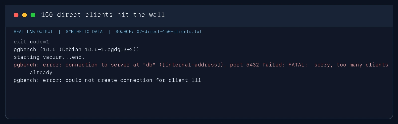
Figure 3: Real lab-output capture; the internal address is redacted. The process exits nonzero, and client 111 receives FATAL: sorry, too many clients already. This is not “a little slower.” The request never enters the database.

A production incident can be worse: once business connections occupy every slot, the DBA’s diagnostic session may be rejected too. Raising max_connections from 100 to 500 in isolation is like seeing a restaurant queue and immediately hiring 400 more waiters. The kitchen did not get larger; now everyone collides inside it.

2.2 One Query Reads Almost 300,000 Rows to Find 30

A slow query rarely writes, “I am slow because an index is missing” in its log line. You infer the cause from its plan, buffer activity, I/O time, call count, and row-estimation errors. The synthetic orders table contains 300,000 rows, while the target predicate matches only 30. Without an appropriate index, PostgreSQL still walks nearly the entire library to retrieve those few books.

2.3 DELETE Is Not a Paper Shredder

PostgreSQL’s MVCC keeps old row versions so concurrent transactions can continue to see a consistent world. An UPDATE usually creates a new version, and a DELETE marks the old version for later cleanup. Imagine a wardrobe: pressing Delete moves clothes into a “to be cleared” compartment; they do not disappear from the apartment at that instant. When autovacuum cannot keep up, table scans, indexes, and disk usage slowly get fatter.

2.4 A Green Backup Job That Nobody Has Restored

A daily green “backup completed” indicator proves only that some files were written. It does not prove that the files are complete, the WAL sequence is continuous, the recovery settings are correct, or the on-call engineer knows which second to stop at. An untested backup is a hope, not a recovery capability.

3. Root Cause: The Team Delivered a Database, but Not Its Safety Nets

These four symptoms are not four unrelated bugs. They share one root cause: the launch checklist tests static state—service starts, endpoint responds, row counts match, configuration loaded—but not the way the system degrades under pressure and human error.

A production database should ship with four safety nets:

1. Traffic safety: application sessions are pooled, rescue connections are reserved, and overload queues or fails quickly in a known way.
2. Evidence safety: pg_stat_statements, slow-query logging, and EXPLAIN (ANALYZE, BUFFERS) turn “it feels slow” into a plan, row count, and I/O trail.
3. Space safety: autovacuum thresholds, duration, freeze age, and dead-tuple trends are visible before cleanup silently falls weeks behind.
4. Time safety: base backups, archived WAL, recovery targets, RPO/RTO, and rehearsal records form one closed loop.

The rest of this article walks through each gate using the measured lab evidence.

4. Gate One: A Connection Pool Is a Flow-Control Valve

PgBouncer transaction pooling can multiplex many client sessions over a smaller number of database connections. It works like the host at a restaurant. One hundred and fifty guests can take queue numbers; the kitchen does not need 150 chefs simultaneously. When one table finishes a transaction, its chef can immediately serve the next table.

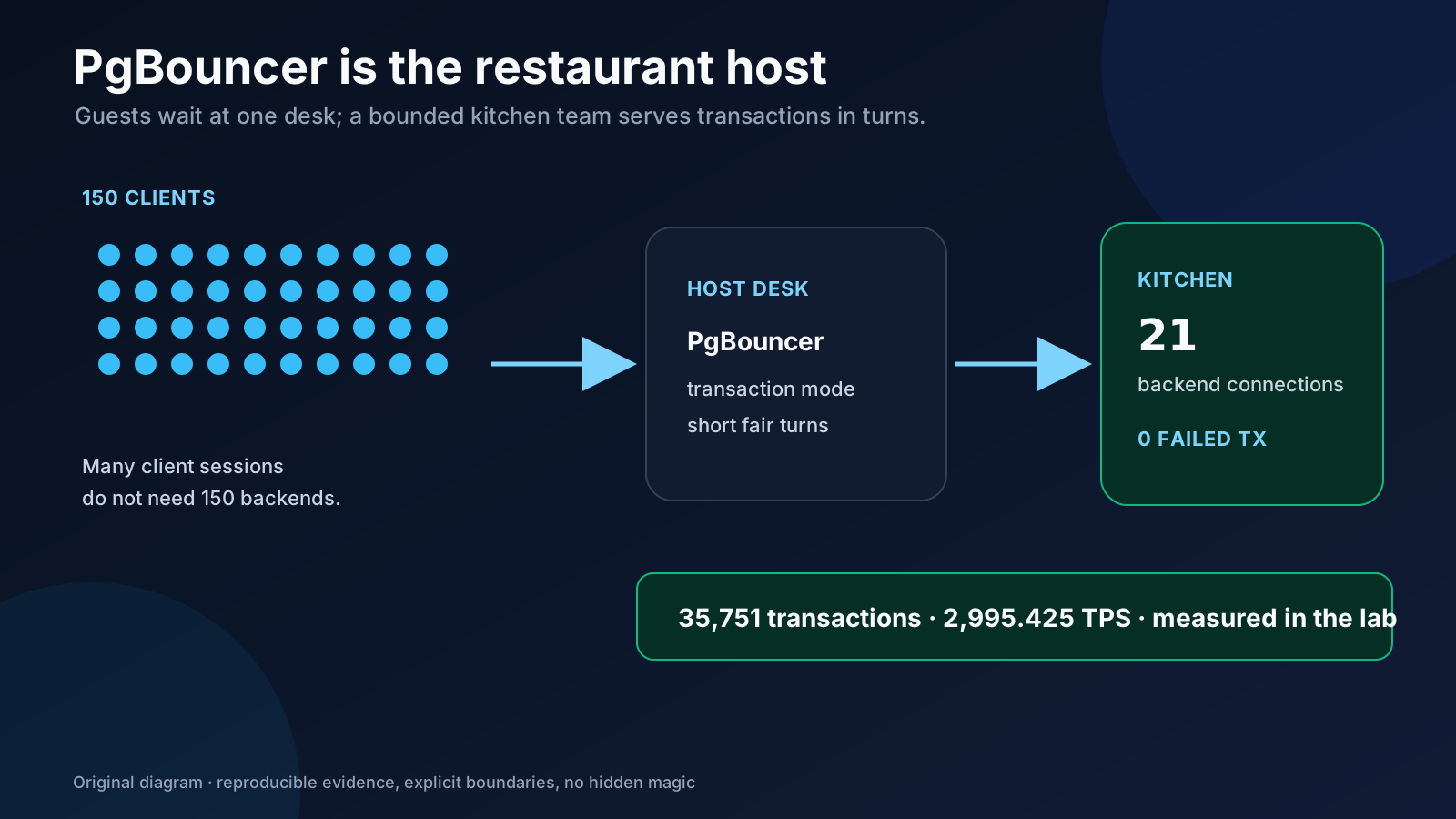
Figure 4: Original diagram. Transaction mode returns a connection after every transaction. Session state, temporary tables, advisory locks, and some prepared-statement patterns therefore require an explicit compatibility review; changing only the endpoint is not an acceptance test.

With the same 150 clients, database, and isolated network, the PgBouncer path behaves differently:

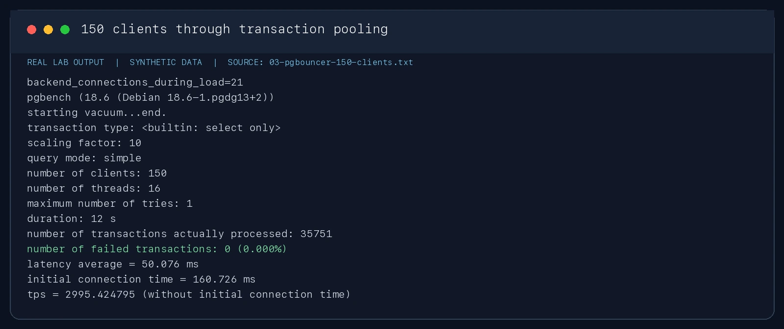
Figure 5: Real lab-output capture. The database has about 21 backend connections during load. Over 12 seconds, the test completes 35,751 read-only transactions, fails zero, averages 50.076ms latency, and reports 2,995.425 TPS. Those figures describe this sandbox—not your capacity.

Before launch, answer at least these questions:

• Are you choosing session, transaction, or statement pooling, and why?
• Does the application depend on long-lived SET state, temporary tables, or session advisory locks?
• Is pool_size derived from database CPU and I/O capacity instead of copied from a random configuration?
• Are operational roles and superuser_reserved_connections or reserved_connections protected?
• Do dashboards show pool wait time, queued clients, and actual database backends together?

The conclusion is not “transaction mode everywhere.” The conclusion is: choose the mode explicitly, then test it against real application behavior.

5. Gate Two: Turn Slow SQL from Guesswork into a Case File

The predicate in this experiment is customer_id = 4241 AND status = 'paid'. Before the index exists, the plan chooses a Parallel Seq Scan:

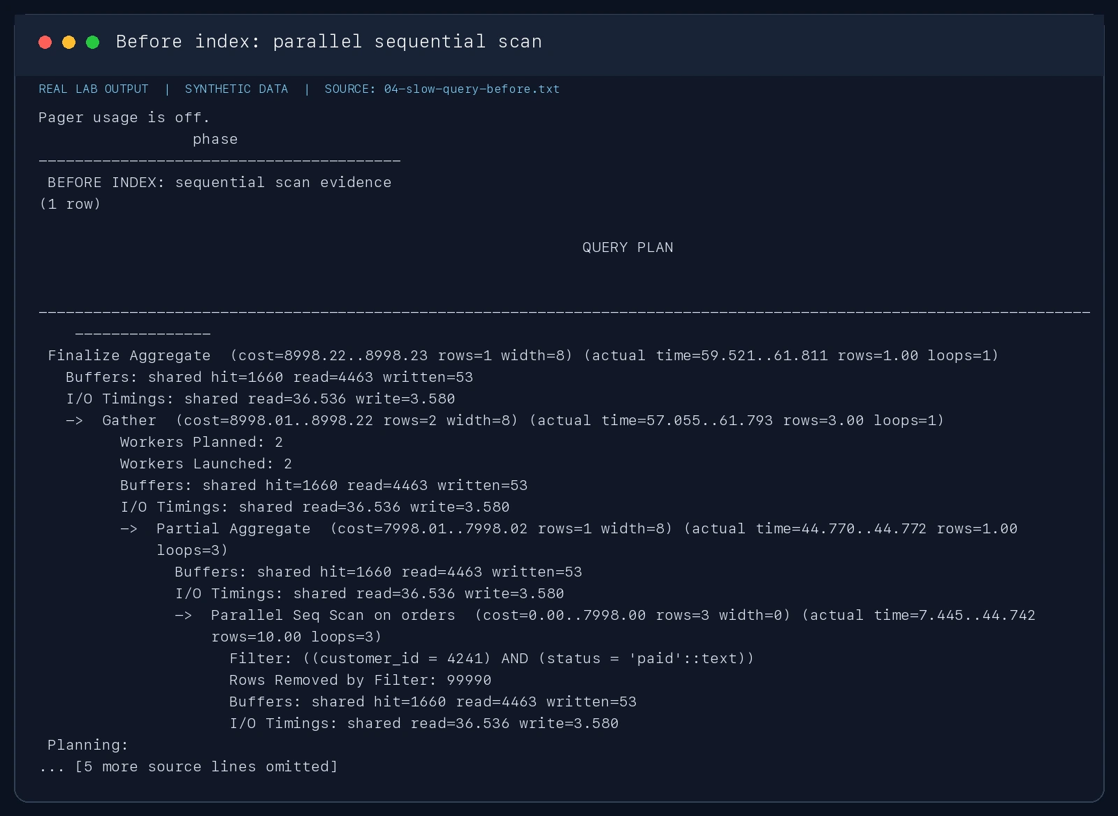
Figure 6: Real lab-output capture. Three execution processes return about ten rows each while each filters roughly 99,990. Total execution time is 61.953ms. “61” is less important than the scan strategy and the number of discarded rows.

The lab then creates a composite index that matches the predicates and runs ANALYZE:

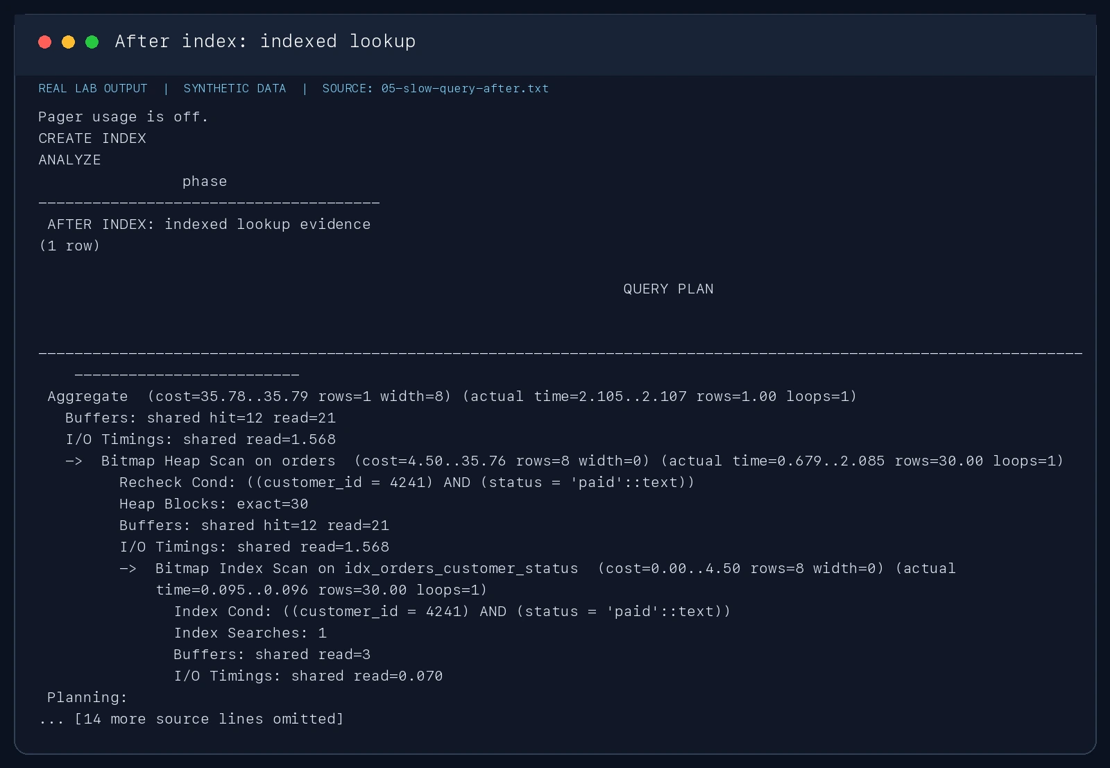
Figure 7: Real lab-output capture. The index finds 30 entries and visits 30 exact heap blocks. Total execution time is 2.153ms, about 28.8 times faster in this run. A different cache state, concurrency level, or data distribution will change the ratio.

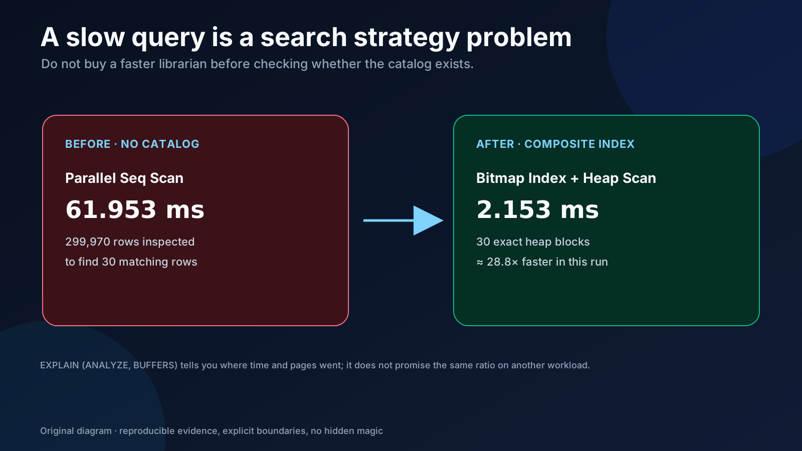
Figure 8: Original diagram. An index is a library catalog, but more catalogs are not automatically better. Every index consumes disk, adds write cost, and requires maintenance. Build indexes for high-value queries supported by evidence.

A disciplined investigation order looks like this:

1. Use pg_stat_statements to find SQL with the most total time, mean time, calls, and temporary blocks. Do not start with a single dramatic log line.
2. Run EXPLAIN (ANALYZE, BUFFERS) on a safe pre-production copy. ANALYZE really executes the statement, so an UPDATE or DELETE needs a rollback wrapper—or plain EXPLAIN only.
3. Compare estimated rows with actual rows. When they differ by orders of magnitude, inspect statistics, skew, and correlated columns before assuming that another index is the only answer.
4. After a change, repeat the same parameters and cache conditions and observe the write penalty. Do not publish only the prettiest run.

pg_stat_statements is an airport’s aggregate delay board: it tells you which route has wasted the most time overall. A slow-query log is one passenger complaint. Both matter, but one complaint alone should not decide whether to build a new runway.

6. Gate Three: Ordinary VACUUM Reclaims Reusable Space

The experiment updates 150,000 rows and deletes 30,000. The statistics view then reports 180,000 dead tuples:

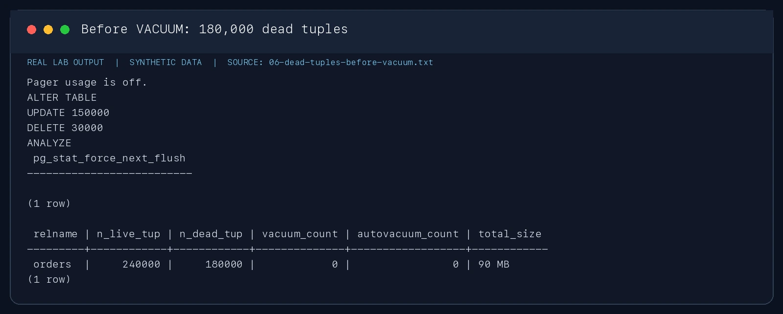
Figure 9: Real lab-output capture. To produce stable evidence, the lab temporarily disables autovacuum for this synthetic table, creates the churn, runs ANALYZE, and flushes statistics. Never leave autovacuum disabled on a production table without a tightly controlled substitute.

After an ordinary VACUUM (ANALYZE):

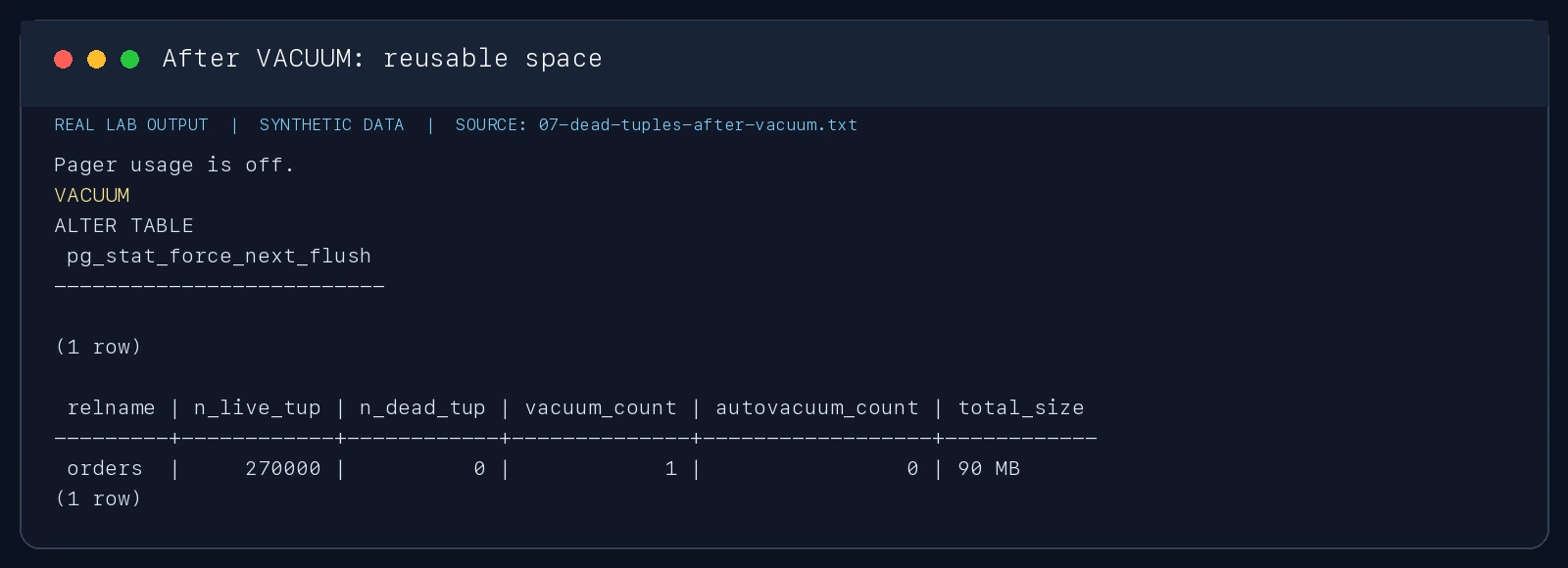
Figure 10: Real lab-output capture. n_dead_tup becomes zero and vacuum_count increases, while total size remains about 90MB. This is useful evidence against the common belief that VACUUM must shrink the file.

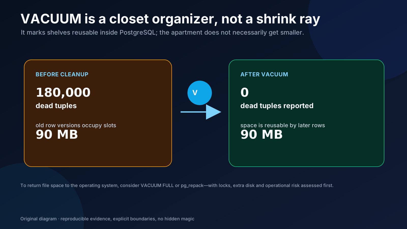
Figure 11: Original diagram. Ordinary VACUUM marks slots reusable inside the relation; it generally does not immediately return trailing file space to the operating system. VACUUM FULL rewrites and locks the table, while pg_repack also requires extra space and an operational review.

Production monitoring must look beyond the current dead-tuple number. Track the trend and its causes: long transactions that hold old snapshots, canceled autovacuum workers, table-specific scale factors for huge relations, and relfrozenxid age approaching dangerous territory. Cleaning is not “the janitor visited once.” It is a continuous balance among customer traffic, garbage generation, and cleanup capacity.

7. Gate Four: Delete Something, Then Turn Back the Clock

PITR works like a video game’s save system. A base backup is a full saved game at one moment. Archived WAL is a move-by-move recording after that point. Recovery loads the save, replays the recording, and presses Pause immediately before the destructive move.

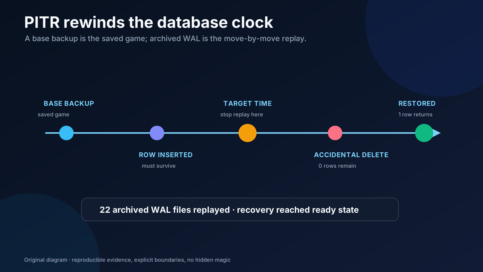
Figure 12: Original diagram. The recovery target must be after the desired transaction and before the accident. Production recovery should normally happen in a side-by-side instance first, rather than turning the only source database into an experiment.

The lab performs these steps: take a base backup; insert a marker row and switch WAL; record a recovery target; delete the marker and switch WAL again; prove the current database contains zero matching rows; stop the source; copy the base backup into a fresh volume; write recovery.signal, restore_command, and recovery_target_time; start an isolated recovery instance; and query the marker row.

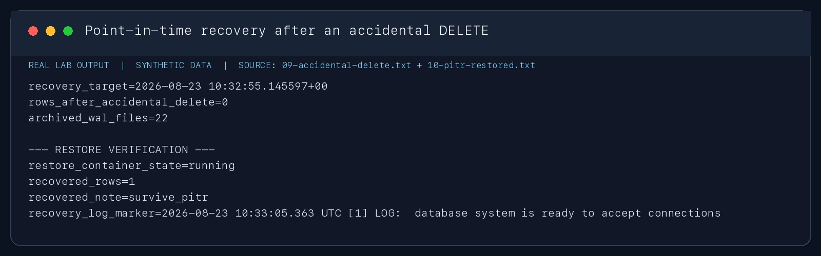
Figure 13: Real lab-output capture. The post-incident query returns zero; the archive contains 22 WAL files; the restored instance reaches running/ready state and returns the marker value. The lab publishes no host port.

This proves that the recovery chain works in the lab. It does not establish a production RTO. A real RTO includes fetching the base backup, downloading archives, replaying a large WAL backlog, validating business invariants, switching connections, and coordinating a decision. A serious acceptance sheet should state:

• RPO: How many minutes of data may be lost, and is archive delay consistently below that limit?
• RTO: How long from declaring recovery until traffic reopens, and what did the latest rehearsal measure?
• Are backups off-site, encrypted, and protected from deletion by the same single administrator?
• Who may start a recovery, who approves it, and who validates critical business data?
• How are timeline forks and the old primary handled so two writable databases cannot reappear?

8. Final Acceptance Is Not One Green “Service Up” Screenshot

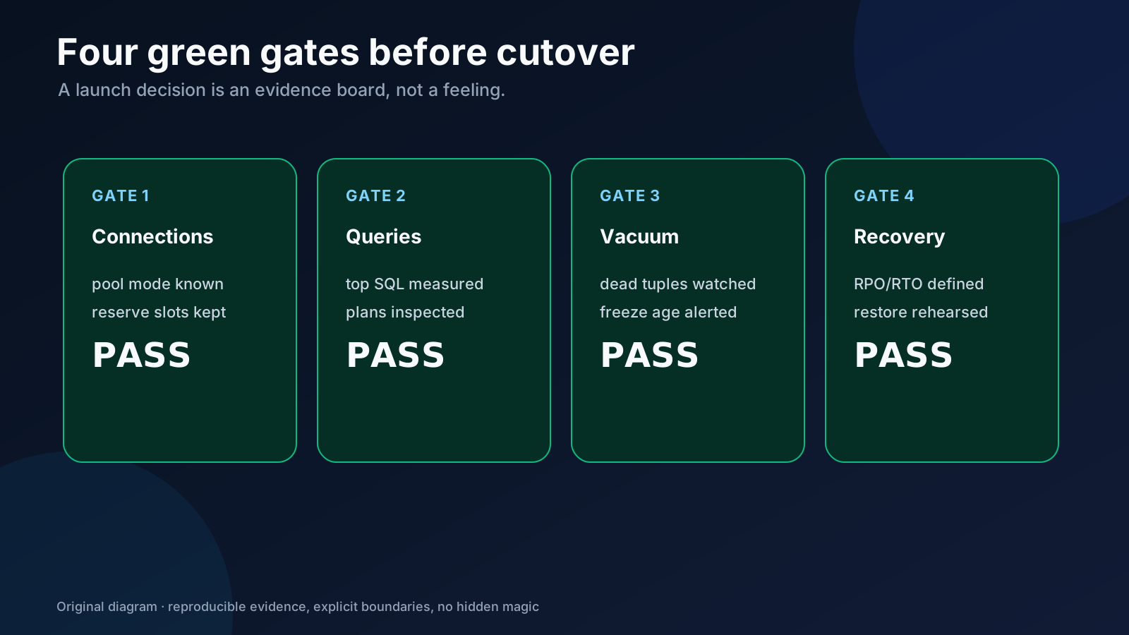
Figure 14: Original diagram. Production readiness means four evidence-backed green gates, not one successful SELECT 1. Any gate without an owner, threshold, and rehearsal record is unknown—not passed by default.

The complete lab writes an acceptance summary at the end:

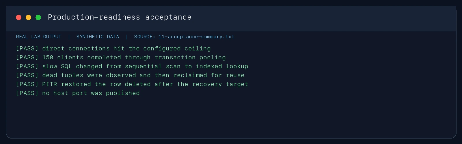
Figure 15: Real lab-output capture. Direct connection ceiling, pooled concurrency, query-plan change, dead-tuple reclamation, PITR recovery, and the no-host-port boundary all pass.

A practical cutover plan operates on several time horizons.

T-30 days: freeze data-type mappings; run top SQL against a production-scale copy; select and test the PgBouncer mode; define RPO/RTO; complete the first recovery rehearsal; alert on dead tuples, freeze age, archive failures, and pool waits.

T-7 days: reconcile row counts, checksums, and business invariants again; load-test pool and reconnection behavior; rehearse rollback; confirm the on-call roster, change window, and connection-string or DNS TTL; keep a read-only window for the old database.

T-0: pause writes or converge the dual-write stream; record the final incremental position; run the final checks; release traffic by percentage; watch errors, pool waits, P95/P99, WAL generation, and replication or archive lag. If a threshold is crossed, follow the agreed rollback rule rather than holding an emergency vote in chat.

T+1 through T+30: do not dismantle the old system immediately; review new query plans, autovacuum behavior, and capacity trends; perform at least one more restore from an actual production backup into isolation. A migration is truly complete when the runbook, alerts, and rehearsals have owners—not merely when the old server is powered off.

9. One-Click Labs: Windows 11, Ubuntu 26.04, and macOS 26

Safety boundary: The package operates only on a fixed lab project, uses synthetic data, loads no real credentials, publishes no host ports, and never runs a global docker system prune. It pulls the official PostgreSQL 18 image and temporarily consumes several hundred megabytes. Do not run two copies against resources with the same lab name.

Download the complete three-platform PostgreSQL readiness lab ZIP. It contains Compose, PgBouncer, SQL, PITR logic, all three entry points, the Agent prompt, and privacy-sanitized reference output. Its SHA-256 is 7b1e0ce68cc52dc36b76cf60bcae6c2e8094153560e2cd7e8536fea66f3cf471.

9.1 Human-Started, Fully Automatic Execution

Windows 11: Docker Desktop must be running Linux containers with WSL 2 integration. Extract the archive and run in PowerShell:

Set-ExecutionPolicy -Scope Process Bypass
.\Run-Windows11.ps1

The entry point is also available directly as Run-Windows11.ps1. It invokes the same run-lab.sh through Windows’ WSL rather than maintaining a reduced PowerShell experiment with subtly different behavior.

Ubuntu 26.04: with Docker Engine and Compose v2 ready:

chmod +x run-lab.sh run-ubuntu-26.04.sh
./run-ubuntu-26.04.sh

Direct entry point: run-ubuntu-26.04.sh.

macOS 26: after starting your local Docker runtime:

chmod +x run-lab.sh run-macos-26.zsh
./run-macos-26.zsh

Direct entry point: run-macos-26.zsh.

All three eventually execute the same run-lab.sh. Success is not merely a zero-looking exit status. Require all six [PASS] lines in results/11-acceptance-summary.txt, then confirm that the scoped containers, network, and volumes were removed.

9.2 Agent-Driven Setup and Acceptance

Give the following instruction to an Agent that is allowed to run local commands. A complete bilingual copy is in AGENT-PROMPT.md:

Run the PostgreSQL production-readiness lab in the current directory without connecting to or changing any existing database. Read the README, Compose file, and current-platform entry point first. Operate only on the fixed lab project and restore container; never publish a host port, load a real credential, or run a global Docker prune. Use the PowerShell entry on Windows 11, Bash entry on Ubuntu 26.04, or zsh entry on macOS 26. After execution, require all six [PASS] lines, check for duplicate side effects, and confirm scoped cleanup. If anything fails, retain the logs and explain the root cause; never rewrite acceptance output to manufacture success.

The Agent method is not valuable merely because it saves three commands. Its value is that authority, success criteria, and failure evidence are explicit before execution. An Agent told only “make PostgreSQL ready” is like a child told “clean the kitchen”: it cannot know which cupboards are forbidden or what “done” means.

10. Q&A

Q1: The 150-client direct test fails. Should I immediately raise max_connections to 300?

Not in isolation. First derive backend concurrency from transaction duration and database CPU/I/O capacity, then fold external sessions through PgBouncer. Preserve operational connections and test the real connection lifecycle. Connections are a budget, not a luxury feature whose value rises with the number.

Q2: Why does the database show about 21 backends for 150 clients instead of a perfectly round configured number?

The snapshot includes load connections, the measurement query itself, and whatever was active at that instant. Transaction pooling creates and reuses backends according to demand; a snapshot is not required to equal the ceiling. The useful evidence is that backend count is dramatically below client count and no transaction fails—not a cosmetically perfect “20.”

Q3: The index made this query 28.8 times faster. Can I create it in production immediately?

Review write amplification, disk capacity, locks, and version capabilities first. Large production tables often use CREATE INDEX CONCURRENTLY, but it runs longer and can leave an invalid index after failure. Monitor it and prepare cleanup. Column order must also fit actual predicates, ordering, and selectivity.

Q4: The file did not shrink after VACUUM. Did VACUUM fail?

No. Ordinary VACUUM primarily makes internal space reusable and maintains visibility information so bloat does not keep growing. Returning space to the operating system is a separate decision. Only when that space will remain unused should you consider an operation that rewrites or relocates data.

Q5: I have cloud-provider snapshots. Do I still need PostgreSQL PITR?

Usually yes. A volume snapshot answers “return this disk to a point,” while database PITR combines a consistent base backup with precise WAL replay. They can complement each other, but cross-volume consistency, WAL location, and the actual restore procedure must be tested.

Q6: The lab recovered successfully. Is my backup strategy now approved?

It proves only that this synthetic recovery mechanism passes. Production acceptance requires measuring RPO/RTO at real backup size, validating business data, testing keys and permissions, rehearsing an off-site failure, and asking someone other than the author to complete the runbook independently.

Q7: Why does the lab not expose a port so I can connect manually?

Its purpose is mechanism verification, not a long-running database deployment. Components communicate inside an isolated Docker network, reducing accidental connections, port collisions, and exposure of deliberately weak lab settings. Read the generated results/ for evidence.

11. References and the Final Sentence

• PostgreSQL 18: The Cumulative Statistics System
• PostgreSQL 18: pg_stat_statements
• PostgreSQL 18: Routine Vacuuming
• PostgreSQL 18: Continuous Archiving and PITR
• PgBouncer: Features and pooling compatibility
• PgBouncer: Usage

This series moved from “why migrate” to “how to migrate,” then from “how to tune” to “how to prove.” If you remember only one sentence from the finale, make it this one: do not ship a database that you have never tried to break and never personally restored.